Having explored the realm of frequency analysis tbrough the Fast Fourier Transform (FFT), where we dissected signals into their constituent frequencies, we now shift our focus to another powerful tool in signal processing: autocorrelation (ACF). While FFT helps us understand the frequency components of a signal, autocorrelation offers a different perspective by measuring how a signal correlates with itself over varying time lags. This self-referential approach doesn’t just complement our frequency-based insights but opens up new avenues for analyzing signal properties such as periodicity, signal similarity over time, and identifying repeating patterns. Autocorrelation, therefore, stands as a crucial technique, especially when the frequency content alone isn’t sufficient to capture the full story of a signal’s behavior.

Example 1: Autocorrelation of Pure Tone

We now consider the autocorrelation of a pure tone signal: \(s(t) = \cos(2\pi \cdot f_0 \cdot t)\)

import numpy as np
from scipy.signal import correlate
from matplotlib import pyplot as plt

fs = 1000
t = np.arange(0, 1, 1/fs)
f0 = 3

s_t = np.cos(2*np.pi*f0*t)

corr = correlate(s_t, s_t, mode='full')
plt.figure(figsize=(10, 8))
plt.subplot(2, 1, 1)
plt.plot(t, s_t)
plt.xlabel('Time [s]')
plt.ylabel('Amplitude')
plt.subplot(2, 1, 2)
plt.plot(corr)
plt.xlabel("Lag")
plt.ylabel("Correlation")

Text(0, 0.5, 'Correlation')

The graph of above correlation is symmetric, which means, again, only half of the information is useful. In common practice, we tend to normalize the highest peak to 1. So a complete version of calculating autocorrelation is as below:

corr = correlate(s_t, s_t, mode='full')
n = len(corr)
corr = corr[n//2:]
# normalize
corr /= corr[0]
plt.figure(figsize=(10, 4))
plt.plot(corr)
plt.xlabel("Lag")
plt.ylabel("Correlation")

Text(0, 0.5, 'Correlation')

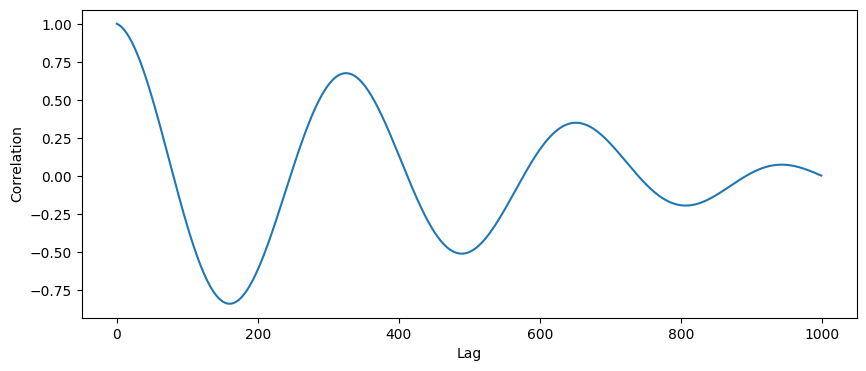
We can observe many peaks on the graph with various lags. Now we need to figure out two things:

• What is the meaning of lag?
• What is the meaning of these peaks?

Example 2: An illustration of the ACF process

Here we illustrate the process of computing ACF. The code below is not required for you. You can execute and watch the generated video.

import numpy as np
import matplotlib.pyplot as plt
from matplotlib.animation import FuncAnimation
from IPython.display import HTML    

# Generate sample time series data
fs = 100
t = np.arange(0, 1, 1/fs)
f0 = 3
s_t = np.cos(2*np.pi*f0*t) 

# Autocorrelation function 
def autocorrelation(x):
    result = correlate(x, x, mode='full')
    result /= np.max(result)
    result = result[result.size // 2:]
    return result

def signal_roll(x, lag, pad_value=0):
    result = np.zeros_like(x)
    if lag > 0:
        result[:lag] = pad_value
        result[lag:] = x[:-lag]
    elif lag < 0:
        result[lag:] = pad_value
        result[:lag] = x[-lag:]
    else:
        result = x
    return result

acf = autocorrelation(s_t)

# Set up the figure with two subplots
fig, (ax1, ax2) = plt.subplots(2, 1, figsize=(12, 10))

# Plotting the original signal
ax1.plot(t, s_t, label='Original Signal', color='red')
line_lagged, = ax1.plot(t, s_t, label='Lagged Signal', color='blue')
ax1.set_title('Signal and Lagged Signal')
ax1.set_xlabel('Time')
ax1.set_ylabel('Amplitude')
ax1.legend()

# Placeholder for the autocorrelation plot
ax2.set_title('Autocorrelation')
ax2.set_xlim(0, len(t))
ax2.set_xlabel('Lag')
ax2.set_ylabel('Autocorrelation')
ax2.set_ylim(-1, 1)
line_autocorr, = ax2.plot([], [], lw=2)
line_autocorrs = []

# Initialize animation
def init():
    line_lagged.set_data([], [])
    line_autocorr.set_data([], [])
    return line_lagged, line_autocorr

# Update function for the animation
def update(lag):
    # Update the lagged signal
    lagged_signal = signal_roll(s_t, lag)
    line_lagged.set_data(t, lagged_signal)
    
    # Calculate and update the autocorrelation plot
    autocorr = acf[lag]
    
    line_autocorrs.append(autocorr)
    lags = np.arange(len(line_autocorrs))
    line_autocorr.set_data(lags, line_autocorrs)
    
    return line_lagged, line_autocorr

max_lag = len(t)   # Max lag is half the signal length to avoid too much empty space
ani = FuncAnimation(fig, update, frames=range(max_lag), init_func=init, blit=True, repeat=False)

# # Display the animation
HTML(ani.to_html5_video())

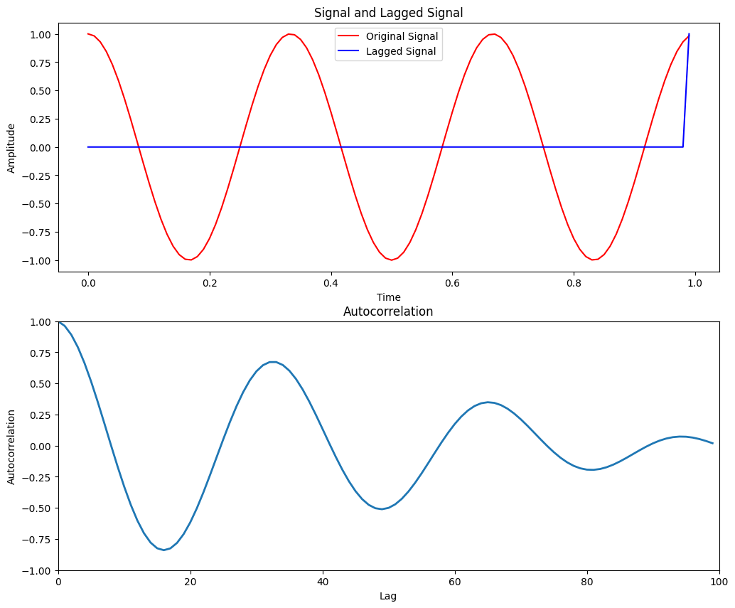
As can be seen from the animation, lag means the step the signal moves. When the signal moves to the positive direction, 0 will be padding in the empty place. And multiplication will be exercised between the “delayed” signal and original signal. Therefore, ACF will observe the largest value at lag=0. At the same time, we will observe peaks at each period point. Intuitively, correlation is an approach for measuring the similarity of two signals. Auto-correlation can be viewed as the special case of correlation, i.e. comparing the shifted version with itself. When there is no shift (lag=0), similarity reaches the maximum value. When lag equals to the periodicity, at least one part of the signal is perfectly matched, thus reaching the peak.

Different from FFT, ACF can only acquire one frequency, namely low frequency. Low frequency indicates the overall trend and periodicty of the signal. The algorithm is both computationally faster and significantly more accurate compared to the FFT, since the resolution is not limited by the number of samples used.

Example 3: Extract the periodicity from ACF

import numpy as np
from scipy.signal import correlate, find_peaks
from matplotlib import pyplot as plt

# Autocorrelation function 
def autocorrelation(x):
    result = correlate(x, x, mode='full')
    result /= np.max(result)
    result = result[result.size // 2:]
    return result

# Generate sample time series data
fs = 100
t = np.arange(0, 1, 1/fs)
f0 = 5
s_t = np.cos(2*np.pi*f0*t) 

acf = autocorrelation(s_t)
x, _ = find_peaks(acf, prominence=0.1)
plt.figure(figsize=(10, 4))
plt.stem(acf)
plt.plot(acf)
plt.plot(x, acf[x], "x", color='red')
plt.xlabel("Lag")
plt.ylabel("Correlation")
x, t[x]

(array([20, 40, 60, 79]), array([0.2 , 0.4 , 0.6 , 0.79]))

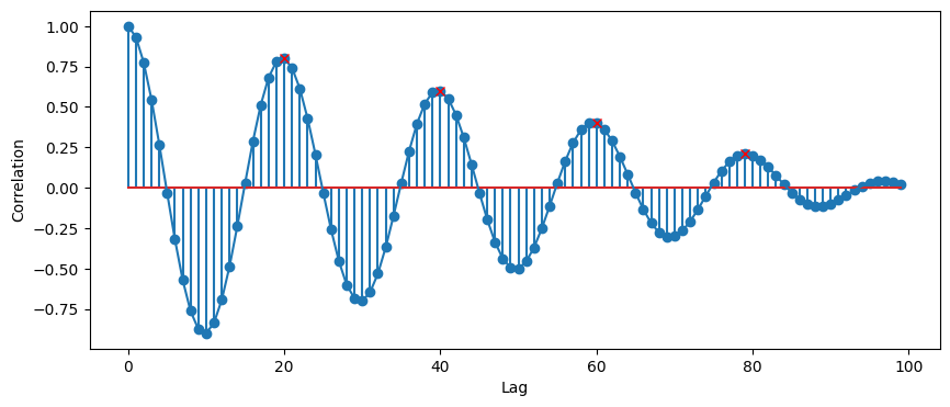
See, peaks will be observed when it reaches its periodicty. As usual, we can use the first peak as the result, which is 0.2s, corresponding to frequency of 5Hz.

Example 4: Adding Windows

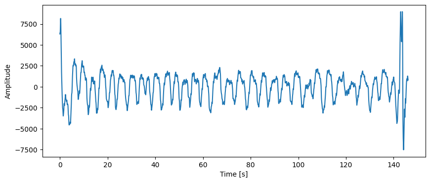
ACF is a time-domain approach, which means it does not transform it to the frequency domain and acquire frequency directly from the time domain. If we want to get more information with the temporal change of frequency, we can use a sliding window along the temporal domain, especially when processing a long time series.

import pickle
from matplotlib import pyplot as plt
br_p = "./example_data/br_0007800f30e4_2023-09-06_15-32-13.pkl"
with open(br_p, "rb") as f:
    br = pickle.load(f)
br_v, fs = br["values"], br["fs"]
print(f"Sampling frequency: {fs} Hz")
br_ts = np.arange(0, len(br_v)/fs, 1/fs)
plt.figure(figsize=(10, 4))
plt.plot(br_ts, br_v)
plt.xlabel("Time [s]")
plt.ylabel("Amplitude")

Sampling frequency: 20 Hz





Text(0, 0.5, 'Amplitude')

window_t = 10 # seconds
window_step = 3 # seconds
window_n = int(window_t * fs)

brs = []
timestamps = []
for i in range(0, len(br_v) - window_n, int(window_step * fs)):
    # print(f"Processing window {i} to {i+window_n}")
    window = br_v[i:i+window_n]
    acf = autocorrelation(window)
    try:
        x, _ = find_peaks(acf, prominence=0.05)
        br = fs / x[0] * 60 # convert to bpm
    except IndexError:
        plt.figure(figsize=(10, 4))
        plt.subplot(2, 1, 1)
        plt.plot(acf)
        plt.subplot(2, 1, 2)
        plt.plot(window)
    t_s = i / fs
    brs.append(br)
    timestamps.append(t_s)
plt.figure(figsize=(10, 4))
plt.plot(timestamps, brs)
plt.xlabel("Time [s]")
plt.ylabel("Breathing Rate [bpm]")

Text(0, 0.5, 'Breathing Rate [bpm]')

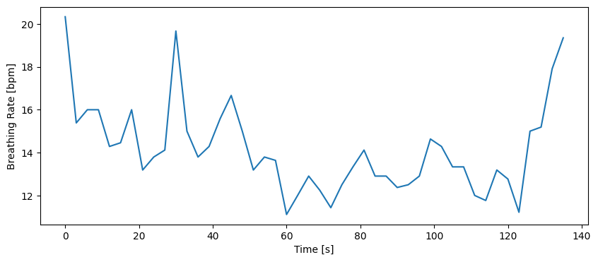
As shown above, we use a window of 10s and time step of 3s to calculate the breathing rate over time, namely $b(t)$. It will result in the time resolution of 3s in $b(t)$. The frequency resolution is determined by the window length, i.e. $1/T$, where $T$ is the window length.

In a nutshell, we introduce ACF in this lab. You are required to know the physical meaning of ACF, get an intuitive understanding of the process of ACF and most importantly, be capable of calculating ACF and periodicity using code.

Programming Task

Task 3-1: Apply ACF (20 points)

You are required to implement the functions in task_3_1.py.

Compute the frequency spectrum of the following signals. You are supposed to implement apply_acf_pt() and apply_acf_pulse() for the following two signals, respectively.

The sampling rate self.fs is 500 Hz. In this task, you are required to return the normalized ACF.

1. Pure Tone: The time range is $0 \le t < 10s$.

1. Pulse signal: The time range is $0 \le t < 2s$.

Task 3-2: Extract Periodicity from ACF (40 points)

You are required to implement the functions in task_3_2.py.

In this task, you are now given multiple files. These files contain signals that we want you to perform frequency analysis on. Your task is to implement get_br_1(), get_br_2(), get_hr_1() and get_hr_2(), respectively.

1. In the following problems, you should use task_3_2_1.pickle. It is a clip of breathing signal. It records the chest movement over time. The sampling rate is 20 Hz. Normally, the breathing rate of an adult is 12-25 BPM. You are required to calculate the breathing rate following the instructions:

   1) get_br_1(): Calculate the breathing rate without windows. You should return the breathing rate (a single float value) in BPM.

   2) get_br_2(): Get the breathing rate over time $b(t)$. You should choose the window length as short as possible with time resolution of 1s. Your window length should be chosen from [1, 10]s and we assume the window length here is an integer.

2. In the following problems, you should use task_3_2_2.pickle. It is a clip of ECG signal after filtering (You do not need to care about it yet.). Your task is to uncover the heart rate from ECG as a function of time. Heartbeat is a periodic event, and the heart rate is the frequency that the heart beats. The heart rate of this participant is between 60 - 120 BPM (Beat Per Minute).

   1) get_hr_1(): You should use a 5-s sliding window with step of 2s.

   2) get_hr_2(): You should adjust your window_length and window_step to make sure the frequency resolution is 0.5 Hz and time resolution is 0.1s.

Note:

• You should use ACF to acquire the results, rather than other approaches. Meanwhile, the accurate answer (Ground Truth, GT) is determined by ACF.
• For task 3_2_1_1, 3_2_2_1 and 3_2_2_2, the answer is fixed. Your answer will be evaluated directly with GT.
• For task 3_2_1_2, you should pick the minimum window length (int) required. You will be graded by the accuracy of your choice of window_length, window_step and your $b(t)$. So will task 3_2_2_1 and 3_2_2_2.

Task 3-3: Data Similarity (40 points)

You are required to implement the functions in task_3_3.py.

Imagine you are the junior technical engineer of a startup company SenseAI, which provides solutions to smart homes with monitoring of temperature, motion, event and sound. One of your customers, Ethan, has installed multiple sensors of your brand in his house. He has been noticing odd patterns—like lights turning on when no one’s home or his heating acting up—and he’s asked SenseAI to analyze the sensor data to figure out what’s going on.

Your boss, Dr. C.S. Wu , assigns you to tackle this problem, using what you have learnt in this lab. You will be given the dataset from Ethan’s apartment. The dataset contains the following signals: motion sensor data, temperature sensor data, event sensor data, and sound sensor data. Before you start, let’s wrap up the concepts you have learnt in this lab.

In class, you’ve used correlation (specifically autocorrelation, ACF) to find repeating patterns in a single signal—like how often a signal oscillates—to calculate frequencies (e.g., breathing or heart rates in Task 3-2). Mathematically, ACF is defined as:

where $\tau$ is the time shift, $N$ is the length of the signal, and $s(t)$ is the signal at time $t$. With correlate(s, s, mode='full'), you get the lags from $-N+1$ to $N-1$, and acf[acf.size//2:] gives you the positive lags ($\tau > 0$).

Now, we’ll use correlation to compare two different signals at the same time (or with shifts) to measure their similarity. Here, we introduce Pearson Correlation Coefficient (PCC) to compare different sensor signals and uncover relationships between them. Pearson measures how linearly two signals move together—perfect for solving Ethan’s mysteries. Here’s the formula:

where $s_1$ and $s_2$ are two signals, and $\bar{s_1}$ and $\bar{s_2}$ are their means. You will find the formula is similar to the correlation formula you have seen above. When $\tau=0$, you will get

This can be seen in the PCC formula above. Specifically, for the numerator, after removing the mean, it is the same as the correlation of two signals (i.e. correlate(s1, s2, mode='full')) and extracting the value at lag 0. For the denominator, it is the square root of the product of the ACF of each signal at lag 0.

Checkpoint 1 (10 points): Implement get_pcc(s1, s2) to calculate the Pearson Correlation Coefficient between two signals. You should return a single float value.

You should use correlate to calculate the PCC. We will delete any scipy.stats.pearsonr or np.corrcoef in your code.

The PCC is a very powerful indicator of similarity between two signals. It ranges from -1 to 1, where 1 means the signals are perfectly correlated, -1 means they are perfectly anti-correlated, and 0 means they are uncorrelated.

You are required to use the PCC / Correlation to solve the following problems.

Note: The sensors are not necessarily working improperly. You should trust your analysis.

You will first work on the motion sensor data. There are two sensors inside the apartment, one in the living room and one in the bedroom. Typically, the light will be turned on when the motion sensor detects movement. When someone is in the living room, we assume that the light in the living room is on. When someone is in the bedroom, we assume that the light in the bedroom is on. We assume that when the person is in the living room, only the motion sensor in the living room will be triggered. The same applies to the bedroom. In other words, the data from the two sensors should be negatively correlated.

Below is an example of the motion sensor data. The sampling rate is 1 Hz.

Checkpoint 2 (5 points): Implement check_motion_sensors(m1, m2) to calculate the PCC between the two motion sensor signals. You should return the PCC value and a Boolean value indicating whether the two sensors are working properly.

You will then work on the temperature sensor data. There are two temperature sensors in the apartment, one in the living room and one in the bedroom. The temperature in the living room and the bedroom should be positively correlated.

Below is an example of the temperature sensor data. The sampling rate is 1 Hz.

Checkpoint 3 (5 points): Implement check_temperature_sensors(t1, t2) to calculate the PCC between the two temperature sensor signals. You should return the PCC value and a Boolean value indicating whether the two sensors are working properly.

On Friday at 11:00 p.m., while he’s at a late study session, his smart home app pings him with an alert: two event sensors—one in the living room near his desk and one by the front door—picked up a sharp crack, like glass breaking. The living room sensor logs it at 11:00:10 p.m., but the door sensor records it at 11:00:10.2 p.m., a 0.2-second mismatch. Ethan’s security system, synced to these sensors, uses sound timing to trigger a break-in alarm and notify the police—but the 0.2-second drift, caused by a recent network lag, risks misclassifying it as two separate noises (e.g., a knock and a crack), delaying the alert. Ethan needs you to sync the signals to confirm it’s one event—a potential break-in—so he can override the system’s confusion, trigger the alarm, and check his door cam footage before someone gets away with his laptop. The threshold for synchronization is 0.1 seconds.

To this end, you will check the two event sensors in the apartment and examine the synchronization between them.

Below is an example of the event sensor data. The sampling rate is 0.1 Hz.

Checkpoint 4 (10 points): Implement sync_event_signals(s1, s2) to synchronize the two sound sensor signals. You should return the delay in seconds and whether it can normally trigger the alarm.

Finally, Ethan’s been puzzled by flickering lights even when he’s away. He suspects a neighbor’s loud music might be triggering the sound-activated lighting system falsely. On Saturday morning, the living room sound sensor records ambient noise, and Ethan provides a known pattern of his neighbor’s bass-heavy music (pattern, 100 samples). You are required to detect the pattern in the sound sensor signal.

Below is an example of the sound sensor data. The sampling rate is 16 kHz.

Checkpoint 5 (10 points): Implement detect_music_pattern(s, p) to detect the neighbor’s music pattern in the sound signal. Use PCC to find where the pattern best matches. Return the starting index (integer) of the strongest match.

You will then report your results to the company’s internal system – Moodle, where your boss and Ethan will see them. Thanks for your efforts!

How to submit

Please run python check.py --uid <YOUR_UID> before submitting. This script performs automated tests on the examples provided in the docstrings. Failing these tests indicates potential critical issues in your code. Strive to resolve these problems. After that, it will create a zip file named after your uid. Make sure you enter the right uid.

It’s important to avoid changing the names of any files, including both the zip file and the program files contained within. Altering file names can lead to grading errors. Ensure that all file names remain as they are to facilitate accurate assessment of your work.

Your submission to Moodle should consist solely of the generated *.zip file. It is your responsibility to double check whether your submitted zip file includes your latest work.